Backfitting algorithm

In statistics, the backfitting algorithm is a simple iterative procedure used to fit a generalized additive model. It was introduced in 1985 by Leo Breiman and Jerome Friedman along with generalized additive models. In most cases, the backfitting algorithm is equivalent to the Gauss–Seidel method algorithm for solving a certain linear system of equations

1 Algorithm
2 Motivation
3 Explicit derivation for two dimensions
4 Issues
5 Modified algorithm
6 References
7 External links

Algorithm

Additive models are a class of non-parametric regression models of the form:

$Y_i = \alpha %2B \sum_{j=1}^p f_j(X_{ij}) %2B \epsilon_i$

where each $X_1, X_2, \ldots, X_p$ is a variable in our $p$ -dimensional predictor $X$ , and $Y$ is our outcome variable. $\epsilon$ represents our inherent error, which is assumed to have mean zero. The $f_j$ represent unspecified smooth functions of a single $X_j$ . Given the flexibility in the $f_j$ , we typically do not have a unique solution: $\alpha$ is left unidentifiable as one can add any constants to any of the $f_j$ and subtract this value from $\alpha$ . It is common to rectify this by constraining

$\sum_{i = 1}^N f_j(X_{ij}) = 0$ for all $j$

leaving

$\alpha = 1/N \sum_{i = 1}^N y_i$

necessarily.

The backfitting algorithm is then:

   Initialize ,
   Do until  converge:
       For each predictor j:
           (a)  (backfitting step)
           (b)  (mean centering of estimated function)

where $\text{Smooth}$ is our smoothing operator. This is typically chosen to be a cubic spline smoother but can be any other appropriate fitting operation, such as:

local polynomial regression
kernel smoothing methods
more complex operators, such as surface smoothers for second and higher-order interactions

In theory, step (b) in the algorithm is not needed as the function estimates are constrained to sum to zero. However, due to numerical issues this might become a problem in practice.^[1]

Motivation

If we consider the problem of minimizing the expected squared error:

$\min E[Y - (\alpha %2B \sum_{j=1}^p \hat{f_j}(x_{ij}))]^2$

There exists a unique solution by the theory of projections given by:

$f_i(X_i) = E[Y - (\alpha %2B \sum_{j \neq i}^p f_j(X_j)) | X_i)]^2$

for i = 1, 2, ..., p.

This gives the matrix interpretation:

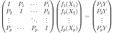
$\begin{pmatrix} I & P_1 & \cdots & P_1 \\ P_2 & I & \cdots & P_2 \\ \vdots & & \ddots & \vdots \\ P_p & \cdots & P_p & I \end{pmatrix} \begin{pmatrix} f_1(X_1)\\ f_2(X_2)\\ \vdots \\ f_p(X_p) \end{pmatrix} = \begin{pmatrix} P_1 Y\\ P_2 Y\\ \vdots \\ P_p Y \end{pmatrix}$

where 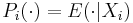$P_i(\cdot) = E(\cdot|X_i)$ . In this context we can imagine a smoother matrix, $S_i$ , which approximates our $P_i$ and gives an estimate, $S_i Y$ , of $E(Y|X)$

$\begin{pmatrix} I & S_1 & \cdots & S_1 \\ S_2 & I & \cdots & S_2 \\ \vdots & & \ddots & \vdots \\ S_p & \cdots & S_p & I \end{pmatrix} \begin{pmatrix} f_1\\ f_2\\ \vdots \\ f_p \end{pmatrix} = \begin{pmatrix} S_1 Y\\ S_2 Y\\ \vdots \\ S_p Y \end{pmatrix}$

or in abbreviated form

$\hat{S}f = QY \,$

An exact solution of this is infeasible to calculate for large np, so the iterative technique of backfitting is used. We take initial guesses $f_i^{(0)}$ and update each $f_i^{(j)}$ in turn to be the smoothed fit for the residuals of all the others:

$\hat{f_i}^{(j)} \leftarrow \text{Smooth}[\lbrace y_i - \hat{\alpha} - \sum_{k \neq j} \hat{f_k}(x_{ik}) \rbrace_1^N ]$

Looking at the abbreviated form it is easy to see the backfitting algorithm as equivalent to the Gauss–Seidel method for linear smoothing operators S.

Explicit derivation for two dimensions

For the two dimensional case, we can formulate the backfitting algorithm explicitly. We have:

$f_1 = S_1(Y-f_2), f_2 = S_2(Y-f_1)$

If we denote $\hat{f}_1^{(i)}$ as the estimate of $f_1$ in the ith updating step, the backfitting steps are

$\hat{f}_1^{(i)} = S_1[Y - \hat{f}_2^{(i-1)}], \hat{f}_2^{(i)} = S_2[Y - \hat{f}_1^{(i-1)}]$

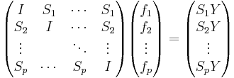
By induction we get

$\hat{f}_1^{(i)} = Y - \sum_{\alpha = 0}^{i-1}(S_1 S_2)^\alpha(I-S_1)Y - (S_1 S_2)^{i -1} S_1\hat{f}_2^{(0)}$

and

$\hat{f}_2^{(i)} = S_2 \sum_{\alpha = 0}^{i-1}(S_1 S_2)^\alpha(I-S_1)Y %2B S_2(S_1 S_2)^{i -1} S_1\hat{f}_2^{(0)}$

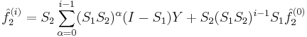
If we assume our constant $\alpha$ is zero and we set $\hat{f}_2^{(0)}= 0$ then we get

$\hat{f}_1^{(i)} = [I - \sum_{\alpha = 0}^{i-1}(S_1 S_2)^\alpha(I-S_1)]Y$

$\hat{f}_2^{(i)} = [S_2 \sum_{\alpha = 0}^{i-1}(S_1 S_2)^\alpha(I-S_1)]Y$

This converges if 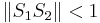$\|S_1 S_2\| < 1$ .

Issues

The choice of when to stop the algorithm is arbitrary and it is hard to know a priori how long reaching a specific conversion threshold will take. Also, the final model depends on the order in which the predictor variables $X_i$ are fit.

As well, the solution found by the backfitting procedure is non-unique. If $b$ is a vector such that $\hat{S}b = 0$ from above, then if $\hat{f}$ is a solution then so is $\hat{f} %2B \alpha b$ is also a solution for any $\alpha \in \mathbb{R}$ . A modification of the backfitting algorithm involving projections onto the eigenspace of S can remedy this problem.

Modified algorithm

We can modify the backfitting algorithm to make it easier to provide a unique solution. Let $\mathcal{V}_1(S_i)$ be the space spanned by all the eigenvectors of S_i that correspond to eigenvalue 1. Then any b satisfying $\ha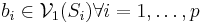t{S}b = 0$ has $b_i \in \mathcal{V}_1(S_i) \forall i=1,\dots,p$ and $\sum_{i=1}^p b_i = 0.$ Now if we take $A$ to be a matrix that projects orthogonally onto 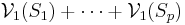$\mathcal{V}_1(S_1) %2B \dots %2B \mathcal{V}_1(S_p)$ , we get the following modified backfitting algorithm:

   Initialize ,, 
   Do until  converge:
       Regress  onto the space , setting 
       For each predictor j:
           Apply backfitting update to  using the smoothing operator , yielding new estimates for

References

^ Hastie, Trevor, Robert Tibshirani and Jerome Friedman (2001). The Elements of Statistical Learning: Data Mining, Inference, and Prediction. Springer, ISBN 0-387-95284-5.

Breiman, L. & Friedman, J. H. (1985). "Estimating optimal transformations for multiple regression and correlations (with discussion)". Journal of the American Statistical Association 80 (391): 580–619. doi:10.2307/2288473. JSTOR 2288473.
Hastie, T. J. & Tibshirani, R. J. (1990). "Generalized Additive Models". Monographs on Statistics and Applied Probability 43.
Härdle, Wolfgang et. al. (June 9, 2004). "Backfitting". http://fedc.wiwi.hu-berlin.de/xplore/ebooks/html/spm/spmhtmlnode37.html. Retrieved 2009-11-15.